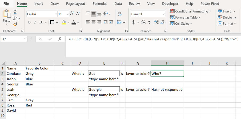
When you are working with a VLOOKUP have you noticed the #NA error if there is no reference or the 0 if there is but no corresponding value? Here is a formula that you can add your own text in for both the #NA error and the 0. Inside the quotation marks is where you would update the text. Has not responded is for 0 and Who? Is for the #NA.
=IFERROR(IF(LEN(VLOOKUP(E2,A:B,2,FALSE))=0,”Has not responded”,VLOOKUP(E2,A:B,2,FALSE)),”Who?”)