This is very similar to SUMIF but we get to evaluate additional criteria in our formula. Here is the same spreadsheet as SUMIF but here we are only getting the sum of the values that match the criteria set by both pieces of the formula.The formula is set up a little differently as well this time.
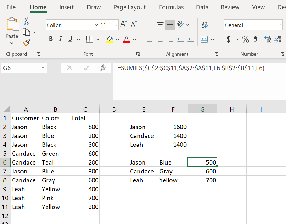
You give the sum range, then the criteria range for the first evaluation followed by the criteria value. You add a comma then give the second criteria range follow by the criteria value for the second evaluation.Here is the formula written out:=SUMIFS($C$2:$C$11,$A$2:$A$11,E6,$B$2:$B$11,F6)We look first at the SUM range for the formula C2:C11. We then state the criteria range for the first evaluation. We are looking for a name in column A so A2:A11. We tell the formula that it is Jason’s name we are looking for by giving E6 as the value. We add a comma and then give the second criteria range for our formula which is colors B2:B11. We then tell the formula that we are looking for the value Blue by giving the formula F6. We get only the sum of Jason – Blue.