Please reach out in you are interested in custom or advanced excel formulas built specifically for your business. Thank you!
Author: DiG with Data
Data Validation for Drop Down Menu in Cell
If you want to get fancy (or, are like me and don’t want people to manually enter values into your spreadsheet because even a space can throw off a VLOOKUP).
You can use Data Validation to create a drop-down menu in a cell.
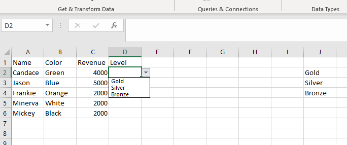
First, create a list of values you want in your drop-down menu. Either on the same sheet you’re working on or on another.
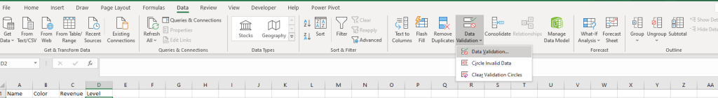
Go to the cell you want to create the drop down in and select it.
Then go to the data tab at the top of the screen and select Data Validation then Data Validation again from the menu.
You will get a Data Validation pop up box. Under the Allow: select List from the menu.
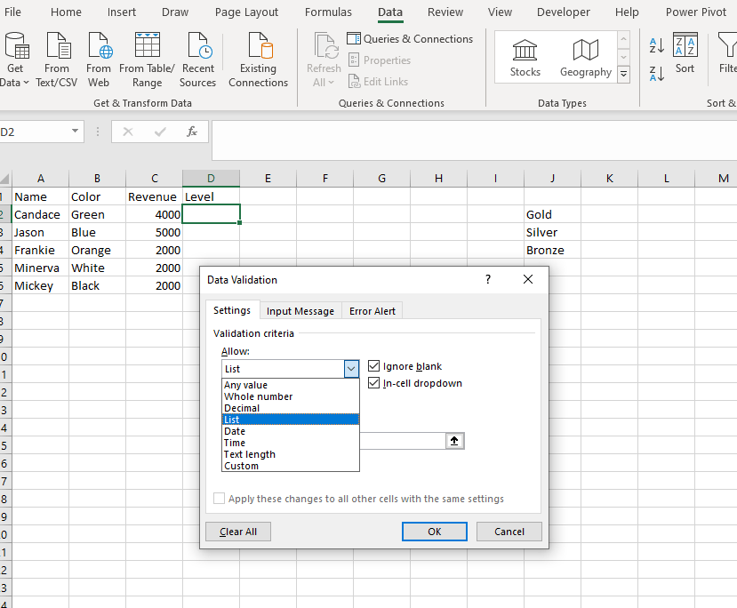
Make sure the boxes for Ignore blank and In-cell dropdown are checked.
Then tell Data Validation where to find your list by clicking on the up arrow in the middle box on the screen.
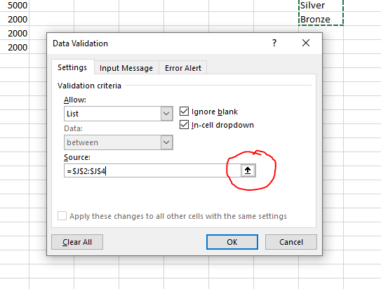
Select the cells in which the list is in (notice these are absolute cell references which means they will not change when you drag, copy and paste or anything else with your data validation cell).
Select OK
Now you have an in cell drop down menu.
INDEX MATCH
First, we will look at the MATCH piece in this formula it returns the position of a value in a range of cells.
In the match you give the value you want the match to find, then the range the value can be found in and how you want the match to evaluate this can be either ascending, descending or exact, we will focus on exact since this is most common and give the formula a 0 which means an exact match. The match formula will return the position
Next is the INDEX piece which will return the specific value of a range that corresponds to the position of the match.
In the index formula you give a range of cells then the row in which you would like returned.
When put these two together you can have your formula look at a value, find that value in a range and then return another value in that same position from another range in table.
How these fit together is by adding the Match formula to the ending value of the index formula. So, where you typically give the index formula the row number you are looking for the match formula is going to provide that.
Here is an example:
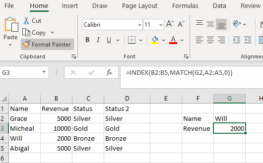
The index is looking in the Revenue column and will return the row that the match gives it based on the Name identified in the cell G2.
XNPV Formula
Anyone that deals with cash flows know that there is not a guarantee that someone will pay on time. Pretend you are a CFO and your company will offer a line of credit to customers to assist in a seasonal business. This means that the company needs to borrow product from your company in July and will pay you back for that product throughout the year. We must figure out how much credit to give them and what the expected return on that should be based on risk.
We use XNVP because this is not a steady cash flow. We have seen the customers books and we can tell when they would likely have the additional capital to pay us back.
Here is the formula
=XNPV(A2,B4:B10,A4:A10)

We offer them the credit in March and figure out a good calculation as to when they can make the rest of their payments based on trends. With the NPV formula it assumes that all of the payments are made evenly whereas this is not the case and customers line of credit should not be impacted based on uneven payment. So, let’s say we know that they can afford a line of credit of $6,000 and realistically pay this back by September first. Great, but we still need to determine how much that is worth today. We know that this is risky but it’s not too risky so we go with 10% today that would be worth $5,802.45 of product to get a return of $6,000.
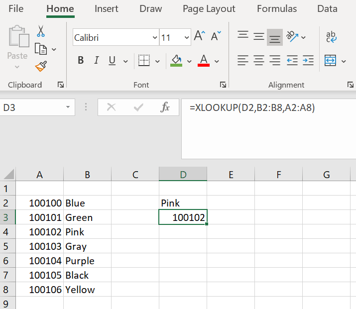
XLOOKUP
This is another formula that is like a VLOOKUP but much more flexible.
In an XLOOKUP you provide the formula with your lookup value. Then give it the lookup range that you want it to find that value in and then the return range. In this formula you can reference the entire column just like the VLOOKUP but you do not have to have the lookup values before the return values.
Here is an example formula:
=XLOOKUP(D2,B2:B8,A2:A8)
And this is it in action:
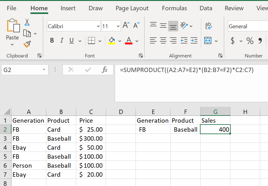
SUMPRODUCT Formula
A formula that evaluates a table to return only the criteria you identify in specific cells.
In this example we are looking in column A to get the generation value, column B to get the product value and then telling the formula where to find the prices which are in column C. We create an input table that holds the values we would like the formula to look for. We are looking in E2 and F2 for these values in our example.
=SUMPRODUCT((A2:A7=E2)*(B2:B7=F2)*C2:C7)
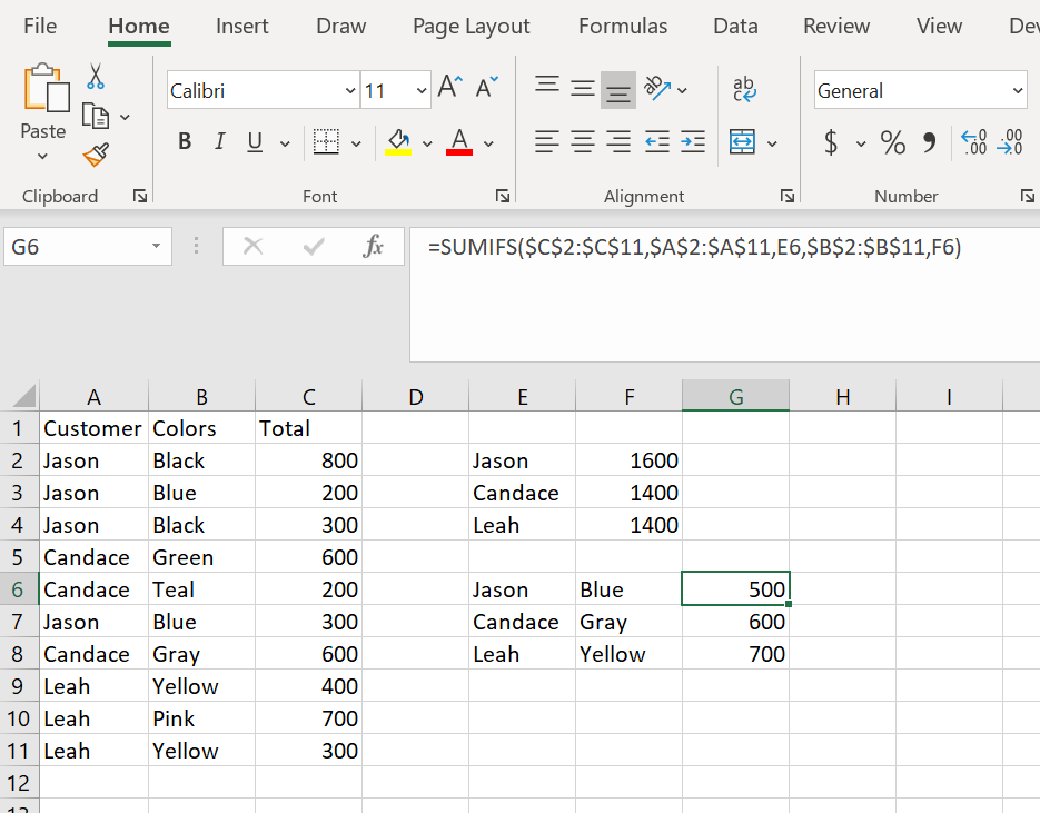
SUMIFS Formula
This is very similar to SUMIF but we get to evaluate additional criteria in our formula. Here is the same spreadsheet as SUMIF but here we are only getting the sum of the values that match the criteria set by both pieces of the formula.The formula is set up a little differently as well this time.
You give the sum range, then the criteria range for the first evaluation followed by the criteria value. You add a comma then give the second criteria range follow by the criteria value for the second evaluation.Here is the formula written out:=SUMIFS($C$2:$C$11,$A$2:$A$11,E6,$B$2:$B$11,F6)We look first at the SUM range for the formula C2:C11. We then state the criteria range for the first evaluation. We are looking for a name in column A so A2:A11. We tell the formula that it is Jason’s name we are looking for by giving E6 as the value. We add a comma and then give the second criteria range for our formula which is colors B2:B11. We then tell the formula that we are looking for the value Blue by giving the formula F6. We get only the sum of Jason – Blue.
SUMIF Formula
SUMIF is a formula that looks at a range of data and will sum only the specified value of that range for you. Here is an example:
=SUMIF($A$2:$A$11,E2,$C$2:$C$11)
This formula is looking at a range of values. You then give it the value that you would like to get the sum of and finally give the formula the range of cells that the values to sum up are in.
We have our customer names in the first column which is our range of values. We want to find the sum of Jason’s Total, so we tell the formula to look at E2. We then select the range of totals.

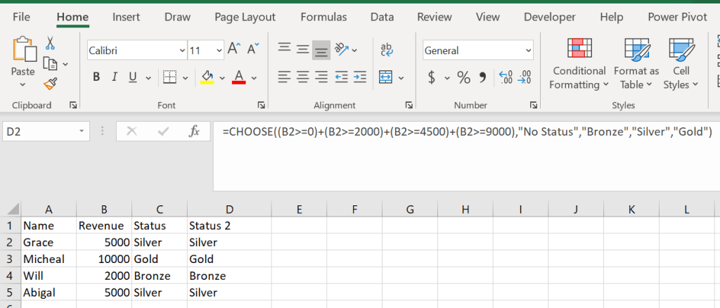
CHOOSE Formula
We generally use nested IF formulas to get values based on conditions, but the CHOOSE function is the best alternative method to get the same result. It is my personal preference to use CHOOSE instead of nested IF formulas because it is easier for me track where I am in my formula without thinking through the false aspect of the formula.
Here is the same table from the nested IF formula but this time we are using CHOOSE.=CHOOSE((B2>=0)+(B2>=2000)+(B2>=4500)+(B2>9000),”No Status”,”Bronze”,”Silver”,”Gold”)CHOOSE is always arranged in ascending order (lowest to highest). In the formula you can see each condition as well as the value that would correspond to that condition.
How this formula works is you give a value to each condition and based on the conditions position the corresponding value is returned.
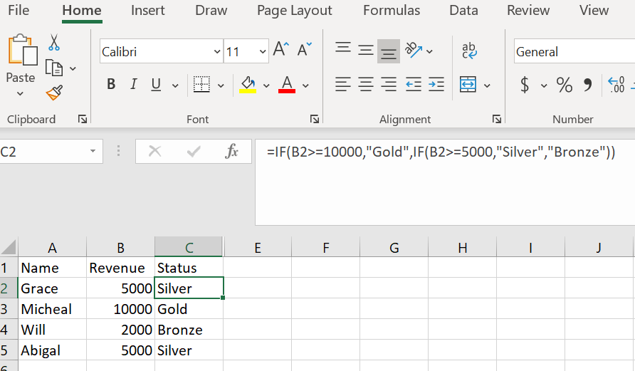
NESTED IF
A nested IF formula is a IF formula inside of another IF formula. This is important when you need to evaluate multiple criteria and the possible outcome for each part of the criteria needs to be different. Here is an example:
=IF(B2>=10000,”Gold”,IF(B2>=5000,”Silver”,”Bronze”))
In this formula we are evaluating our customers revenue to determine what Status we should give them.
In plain language this formula is saying:
If the revenue amount in cell B2 is greater than or equal to 10,000 the customers status should be Gold.
If it’s not but, IF it is greater than or equal to 5,000 it should be Silver.
And if its neither of those then it should be Bronze.
The best practice for writing a nested IF is to always go from largest to smallest value.