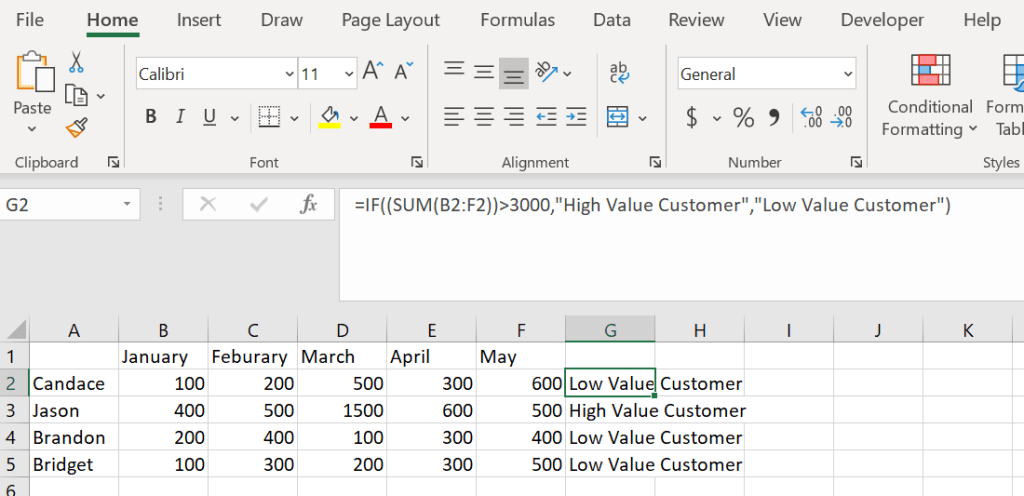
This is an IF formula explained. I wanted to touch on some simple formulas before I started referencing them in more complex ones. An IF formula evaluates a logic test and returns a value for true and false. In this example I want to include a sum formula inside of the logic test portion of the IF formula to get everyone used to seeing how powerful formulas can be when a few are combined.

=IF((SUM(B2:F2))>3000,”High Value Customer”,”Low Value Customer”)

Copying a sheet from one workbook into another.

Sheets of a workbook can be moved or copied into another open workbook or a new workbook without needing to copy over all the data within the spreadsheet.

First go to the bottom of your workbook to the sheet you would like to move or copy and right click. Select the “Move or Copy…” option as shown in the photo.

You will see a list of all the Sheets in that workbook but if you select the drop down next to the name of your workbook you will see all open workbooks as well as a (new book) option. I attached a screenshot to explain.

Select the workbook you would like to move that sheet into whether it be a new one or another open one. Then decide if you would like to move the sheet entirely or if you would like to create a copy (you create a copy by checking the box) of that sheet into the other location. Then simply select OK.

This one is a little different then my others since it is not a formula. Transpose Paste is to take the data from columns and rows and switch their position. So the columns become the rows and the rows become the columns.

This is as simple to do as copying your data (highlight the data and then Ctrl+C), choosing the cell you want to start the transposed data in, right click and under paste selecting the transpose option.

Here are is a screenshot to show you which paste is transpose and also a screenshot of transposed data.

In this formula you are taking the contents from different cells and putting them together into one cell with space included. To accomplish this, you use the ampersand (&) sign to combine text and quotations (” “) with a space between them to show spacing.

This is what your formula will look like

=A1&” “&B1&” “&C1&”.”

If you need to add an additional word to your work here is what that formula will look.

=A2&” “&”just”&” “&B2&” “&C2&”.

When you are working with a VLOOKUP have you noticed the #NA error if there is no reference or the 0 if there is but no corresponding value? Here is a formula that you can add your own text in for both the #NA error and the 0. Inside the quotation marks is where you would update the text. Has not responded is for 0 and Who? Is for the #NA.

=IFERROR(IF(LEN(VLOOKUP(E2,A:B,2,FALSE))=0,”Has not responded”,VLOOKUP(E2,A:B,2,FALSE)),”Who?”)

In a VLOOKUP you can reference the entire column for the table array to make your formula cleaner and easier to move between rows and columns without needing the $ absolutes for specific cell values. (This would be good when you do not have any data underneath your table that you would not want the vlookup to find.)

=VLOOKUP(E5,A:B,2,false)

There are easy formulas to make the letters in your cell UPPER CASE (LIKE THIS), lower case (like this) and Proper Case (Like This) but what if you need Sentence case (Like this)?

=UPPER(LEFT(A1,1))&LOWER(RIGHT(A1,LEN(A1)-1))